
While I’ve long advocated the use of Coefficient of Variation (CV) as a quick and dirty indicator of the forecastability of a time-series, its deficiencies are well recognized. It is true that any series with extremely low CV can be forecast quite accurately (using a moving average or simple exponential smoothing — or even a random walk!). But there are plenty of examples of series with high CV that are also forecastable with good accuracy. Thus:
Low CV => Easy to get accurate forecasts
High CV => Probably worse forecasts, but may still be possible to get good accuracy
If the high CV is due to recurring seasonality, this is “signal” in the data that we should be able to capture in our forecasting model.
An example from early in my industry career was when I did forecasting for a processed meats manufacturer based in the US. (While I won’t identify the company, I can tell you that their bologna has a first name. And if I were one of their most popular products, everyone would be in love with me.)
Hot dog sales were higher in the summer, lower in the winter, and had three huge spikes for the US holidays Memorial Day, Independence Day, and Labor Day. While the seasonality and holiday spikes drove up the volatility of sales, this pattern repeated every year, and we could easily accomodate it in our models and manual overrides. While forecast accuracy was not as good as for very simple demand patterns (we never knew how high the spikes would be), it was much better than the high CV would suggest.
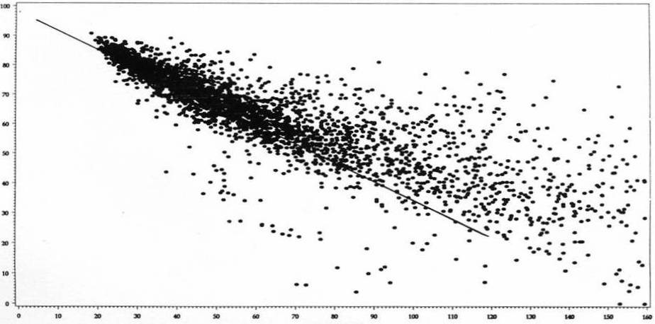
Comet Chart – Forecast Accuracy vs. Volatility
While CV (and the very informative “comet chart” — see above or an example from Sean Schubert on slide 15) gives us a general sense of forecastability, it does not answer the question “What is the best my forecasts can be?” So let’s return to Steve Morlidge’s new approach.
How Good is a “Good” Forecast?
Steve sent me a nice summary of the line of reasoning so far:
- All extrapolation based forecasting is based on the assumption that the signal evident in history will continue into the future.
- This signal is, however, obscured by noise.
- Forecasting algorithms seek to identify the signal and extrapolate it into the future.
- A ‘perfect’ forecast will match the signal 100% but, by definition, can never forecast noise.
- If we understood the nature of the relationship between the signal and noise in the past data we should therefore be able to determine the limits of forecastability.
- Because the naïve forecast uses the current period actual to forecast the next period, the mean naïve forecast error captures what we need to know about the data series we are seeking to forecast; specifically the level of noise and changes in the signal
- Based on this analysis we can make the conjecture that:
- If we knew the level of the noise (OR the nature of changes to the signal) we should be able to determine the ultimate limits of forecastability
- The limit of forecastability can only be expressed in terms of the ratio of the actual forecast error to the naïve forecast error (Relative Absolute Error). This is neat as we already know the upper bound of forecastability can be expressed in these terms (it has a RAE of 1.0)….and it ties in with the notion of FVA!!
At this point, Paul Goodwin of the University of Bath steps in with a mathematical derivation of the “avoidability ratio.” (Paul was recently inducted as a Fellow of the International Institute of Forecasters, and delivered the inaugural presentation “Why Should I Trust Your Forecasts” in the Foresight/SAS Webinar Series.) His assumptions:
- We have the perfect forecasting algorithm
- The remaining errors are pure noise (in the statistical sense that they are stationary and iid with a mean of zero)
- The change in the signal from period to period is unaffected by the previous period’s noise
Under these assumptions:
When the pattern in the data is purely random, the ratio of the variance (MSE) from a perfect algorithm to the MSE of a naive foreast will be 0.5; that is, the perfect algorithm will cut observed noise (using the MSE measure) in half. Using the more practical measure of the ratio of the mean absolute error (MAE), a “perfect” algorithm would never achieve a ratio lower than 0.7 (=√0.5).
What does this mean, and what is the empirical evidence for this approach? We’ll explore the details in Part 3, and make a call to industry for further data for testing.
![]()