We have already discussed feature selection and features reduction, and all the techniques we explored were strictly related and applicable only in the text mining domain.
We have already discussed feature selection and features reduction, and all the techniques we explored were strictly related and applicable only in the text mining domain.
I would like to show you one very powerful method, easy to implement and extremely general, because it is not related to the nature of the problem.
The method is known as coefficients of constraint (Coombs, Dawes and Tversky 1970) or uncertainty coefficient (Press & Flannery 1988) and it is based on the Mutual Information concept.
Mutual Information
As you know, the Mutual Information between two random variables X and Y I(X,Y) measures the uncertainty of X knowing Y, and it says how much the uncertainty (entropy) of X is reduced by Y.
This is more clear looking at the below formula:
I(X,Y)= H(X)-H(X|Y)
Where H is the Entropy functional.
As usual, I don’t want enter in theoretical discussions, but I heartily recommend a deep read of the book
Elements of Information Theory: In my opinion it’s the best book in that field.
Let’s now rethink the mutual information as a measure of “how much helpful is the feature X to classify documents having label L“:
I(L,X) = H(L)-H(L|X)
So, for each label and each features we can calculate the features ranking!
Of course you can consider the average of I(L_i,X) for each label L_i, or also more complex function over that. BTW you have to assign higher rank to the feature Xj that maximize all I(L_i,Xj).
Uncertainty coefficient
Consider a set of people’s data labelled with two different labels, let’s say blue and red, and let’s assume that for this people we have a bunch of variables to describe them.
Moreover, let’s assume that one of the variables is the social security number (SSN) or whatever univocal ID for each person.
Let me do some considerations:
- If I use the SSN to discriminate the people belonging to the red set from the people belonging to blue set, I can achieve 100% of accuracy because the classifier will not find any overlapping between different people.
- Using the SSN as predictor in a new data set never seen before by the classifier, the results will be catastrophic!
- The entropy of such variable is extremely high, because it is almost a uniform distributed variable!
The key point is: the SSN variable could have a great I value but it is dramatically useless to classification job.
To consider this fact in the “mutual information ranking”, we can divide it by the entropy of the feature.
So features as SSN will receive lower rank even if it has an high I value.
This normalization is called uncertainty coefficient.
Comparative Experiment
Do you have enough about the Theory? I know that … I did all my best to simplify it (maybe to much…).
I did some tests on the same data set used in this paper by Berkley University:
In this test the authors did a boolean experiment over
REUTERS data set (actually it is very easy test) and they compared the accuracy obtained using all the words in the data set as features and the features extracted through a Latent Dirichlet Allocation method.
The data set contains 8000 docs and 15818 words. In the paper they claimed that they reduced the feature space by 99.6% and they used the entire data set to “extract” the features.
Under this condition they tested using no more than 20% of the data set as training set.
In the comparative test I focused on the second experiment mentioned: GRAIN vs NOT GRAIN.
Here you are the process I followed:
- I choose as training set 20% of the docs.
- from the above training set I extracted (after stemming and filtering process) all the words and I used them to build the boolean vectors.
- I ranked the words through the uncertainty coefficient.
- I extracted the first 60 features: that is only 0.38% of the original feature space
- I trained an SVM with a gaussian kernel and very high value of C
- I tested over the remaining 80% of the data set.
Before the results, let me show you some graph about the feature ranking.
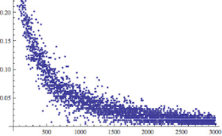 |
| Entropy of the first 3000 features. |
The above graph shows the entropy of the first 3000 features sorted by TF-DF score.
As you can notice, the features having low score have low entropy: it happens because these features are present in really few documents so the distribution follows a Bernulli’s distribution having “p” almost equal to 0: basically the uncertainty of the variable is very small.
Here you are the final ranking of the first 2500 features.
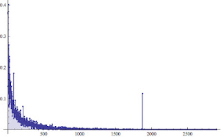 |
| Uncertainty coefficient for all features. |
Results
The overall accuracy measured over the test set is equal to 96.89% and it has been depicted in the below graph (I used their original graph [figure 10.b] as base) as a red circle:
 |
| Accuracy comparison: the red circle represents the accuracy obtained training an SVM with the features extracted through the Uncertainty Coefficients. |
I would like to remark that the features has been extracted using just the training set (20% of the data set), while the experiments done by the authors of the mentioned paper used the entire data set.
Better results can be easily achieved using the conditioned entropies in an iterative algorithm where the mutual information is measured respect a local set of features (adding the features that maximize the M.I. of the current set of features).
Our experiment shows clearly that the “Uncertainty Coefficients” criteria is a really good approach!
Soon, we will see how to use this criteria to build a clustering algorithm.
As usual: stay tuned.
cristian